12.2.7 Measuring Half-Life

Measuring Half-Life

Half-life is defined as:

The time taken for the initial number of nuclei to halve for a particular isotope

This means when a time equal to the half-life has passed, the activity of the sample will also half
This is because the activity is proportional to the number of undecayed nuclei, A ∝ N

Half-life Graph, downloadable IGCSE & GCSE Physics revision notes

When a time equal to the half-life passes, the activity falls by half, when two half-lives pass, the activity falls by another half (which is a quarter of the initial value)

To find an expression for half-life, start with the equation for exponential decay:

N = N₀e^–λt

Where:
- N = number of nuclei remaining in a sample
- N₀ = the initial number of undecayed nuclei (when t = 0)
- λ = decay constant (s^-1)
- t = time interval (s)

When time t is equal to the half-life t_½, the activity N of the sample will be half of its original value, so N = ½ N₀

Calculating Half-Life equation 1

The formula can then be derived as follows:

Calculating Half-Life equation 2

Calculating Half-Life equation 3

Calculating Half-Life equation 3a

Therefore, half-life t_½ can be calculated using the equation:

Calculating Half-Life equation 4

This equation shows that half-life t_½ and the radioactive decay rate constant λ are inversely proportional
- Therefore, the shorter the half-life, the larger the decay constant and the faster the decay

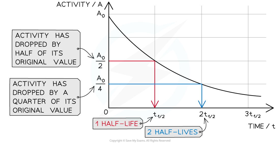
The half-life of a radioactive substance can be determined from decay curves and log graphs
Since half-life is the time taken for the initial number of nuclei, or activity, to reduce by half, it can be found by
- Drawing a line to the curve at the point where the activity has dropped to half of its original value
- Drawing a line from the curve to the time axis, this is the half-life

A linear decay curve. This represents the relationship: $\frac{∆ N}{∆ t} = - λ N$

Measuring Long Half-Lives

For nuclides with long half-lives, on the scale of years, this can be measured by:
- Measuring the mass of the nuclide in a pure sample
- Determining the number of atoms N in the sample using N = nN_A
- Measuring the total activity A of the sample using the counts collected by a detector
- Determining the decay constant using $λ = \frac{A}{N}$
- Calculating half-life using $t_{\frac{1}{2}} = \frac{\ln 2}{λ}$

Note: The sample must be sufficiently large enough in order for a significant number of decays to occur per unit time so that an accurate measure of activity can be made

Measuring Short Half-Lives

For nuclides with short half-lives, on the scale of seconds, hours or days, this can be measured by:
- Measuring the background count rate in the laboratory (to subtract from each reading)
- Taking readings of the count rate against time until the value equals that of the background count rate (i.e. until all of the sample has decayed)
- Plotting a graph of activity, A, against time, t (as corrected count rate ∝ activity, A)
- Making at least 3 estimates of half-life from the graph and taking a mean

- Plotting a graph of ln N against time, t (as corrected count rate ∝ number of nuclei in the sample, N)
- Finding the gradient of this graph, which gives –λ
- Calculating half-life using $t_{\frac{1}{2}} = \frac{\ln 2}{λ}$

Straight-line graphs tend to be more useful than curves for interpreting data
- Due to the exponential nature of radioactive decay logarithms can be used to achieve a straight line graph
Take the exponential decay equation for the number of nuclei

N = N₀ e^–λt

Taking the natural logs of both sides

ln N = ln (N₀) − λt

In this form, this equation can be compared to the equation of a straight line

y = mx + c

Where:
- ln (N) is plotted on the y-axis
- t is plotted on the x-axis
- gradient = −λ
- y-intercept = ln (N₀)

Half-lives can be found in a similar way to the decay curve but the intervals will be regular as shown below:

Half Life Decay Curves 2, downloadable AS & A Level Physics revision notes

A logarithmic graph. This represents the relationship: $\ln N = - λ t + \ln N_{0}$

Note: experimentally, the measurement generally taken is the count rate of the source
- Since count rate ∝ activity ∝ number of nuclei, the graphs will all take the same shapes when plotted against time (or number of half-lives) linearly or logarithmically

Worked example

Strontium-90 is a radioactive isotope with a half-life of 28.0 years. A sample of Strontium-90 has an activity of 6.4 × 10⁹ Bq.

(a)

Calculate the decay constant λ, in year^–1, of Strontium-90.

(b)

Determine the fraction of the sample remaining after 50 years.

Part (a)

Step 1: List the known quantities

- Half-life, t_½ = 28 years

Step 2: Write the equation for half-life

$t_{\frac{1}{2}} = \frac{\ln 2}{λ}$

Step 3: Rearrange for λ and calculate

$λ = \frac{\ln 2}{t_{\frac{1}{2}}} = \frac{\ln 2}{28}$ = 0.025 year⁻¹

Part (b)

Step 1: List the known quantities

- Decay constant, λ = 0.025 year⁻¹
- Time passed, t = 50 years

Step 2: Write the equation for exponential decay

$N = N_{0} e^{- λ t}$

Step 3: Rearrange for $\frac{N}{N_{0}}$ and calculate

$\frac{N}{N_{0}} = e^{- λ t}$

$\frac{N}{N_{0}} = e^{- (0.025) \times 50}$ = 0.287

- Therefore, 28.7% of the sample will remain after 50 years

Worked example

The radioisotope technetium is used extensively in medicine. The graph below shows how the activity of a sample varies with time. Worked Example - Half Life Curve, downloadable AS & A Level Physics revision notes